

Model Assumptions
The model shown here is a model of carbon-dioxide in a static troposphere-like system, i.e., one could consider it a model of carbon dioxide diluted in a non-absorbent medium (for example nitrogen and oxygen) that has the average temperature and pressure profile of the mid-latitude troposphere. The scale height is taken as 8435 m, and the lapse rate is assumed to be 6.5 K/1000 meters. The pressure and temperature of each layer are taken as the pressure and temperature at the middle of that layer. The previous post explains these profiles in more detail. The model treats the earth as a blackbody at 288 K. The model shows the spectrum as it would be seen by an observer at a given altitude looking down at the earth; it is a model of upwelling radiation. The carbon dioxide spectrum is taken from the NIST Webbook. This model is intended to be simple and the results were obtained with a PC program.
Model Caveats and Weaknesses
The model only included carbon dioxide; it does not include other infrared absorbing species in the troposphere. The model only treats absorption and emission; it does not treat scattering and reflectance. The earth is treated as a blackbody at 288K instead of using the actual emission spectrum of the earth. The model uses a moderate-resolution spectrum of carbon dioxide, it would be better to use a high-resolution spectrum such as one from the HITRAN database. the model is static: it does not account for weather patterns, variation withing the troposphere, or geographical factors. The model also does not account for the fact that the earth is warming; it shows results assuming that the temperature profile of the earth does not change. In the future, I may improve this model by accounting for some of these factors (as indicated toward the end of this post), but at some point, it is more reasonable to use models that have already been developed.
Additionally, the model does not account for spectroscopic effects such as pressure broadening, Doppler broadening, or changes in the rotational distribution of the ground vibrational state with temperature. These spectroscopic effects are actually very important in quantitatively understanding how much energy the atmosphere absorbs.
Bear in mind the the point of this model is conceptual and that simplicity is easier to conceptualize.
Model Construction
I built the model on my home PC using Wavemeterics Igor Pro scientific graphing and data analysis program. The model runs in seconds depending on the number of layers used.
Pressure
Pressure is in atmospheres (atm) assuming that the pressure is 1 atm at the earth's surface. Pressure (P) is modeled as:
P = exp(-Z/H)
where Z is the altitude in meters of the middle of a layer and H is the scale height, 8435 m.
Temperature
Temperature (T) is in Kelvin (K) and modeled as:
T = 288 - 6.5*Z/1000
Absorbance
The absorptivity (α) is calculated from the NIST Webbook as explained in a previous post. The Absorbance is calculated as:
A = αCLP
L is the thickness of a layer in meters, C is the volumetric mixing ratio in parts-per million (ppm). The mixing ratio is held constant throughout the troposphere but it is scaled by the pressure (P) in atmospheres to account for the fact that there are fewer absorbers in the same volume at lower pressure.
Transmittance
The transmittance (τ) is calculated from the Beer-Lambert Law as:
τ = 10 - A
Note that the absorptivity was also calculated in log-based 10 units.
Radiance Through a Layer
The radiance through a layer (and incident on the next layer) was calculated analogously to the two-layer model:
In+1 = IBB + τn(In -IBB)
in which IBB is the radiance of a blackbody at the temperature in the middle of the layer,τn is the transmittance of layer n, and In is the radiance incident upon layer n. In the zeroth layer In is taken to be a blackbody at 288 K.
Brightness Temperature
The brightness temperature is calculated as a function of wavelength as the temperature of a blackbody having the same radiance at that wavelength. The brightness temperature contains the same information as a radiance spectrum, but it is easier to visualize the differences because the dynamic range is smaller on a graph.
Running the Model
Optimizing the Number of Layers
The more layers used, the closer the model becomes to a continuous model, i.e., the more accurate the result. Of course adding more layers increases the computation time, but that is not really an issue for a model this simple. Consider an observer at a given height above the earth, looking down. The distance between the observer and the earth is divided into layers, the more layers there are, the smaller each layer is. For example, imagine that the observer is at 10,000 m, and one chooses either a single layer or ten layers. The graph below shows the relationship between the height of a layer and the number of layers.

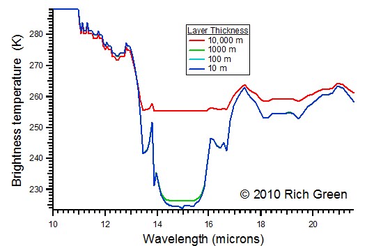
Notice that using too few layers, blunts the fidelity of the model. Whereas using a single layer 10,000 m thick shows near total saturation toward longer wavelength, using more layers shows more of the spectral structure.
Observer Height
Now consider changing the height if the observer. Imagine riding up in a balloon to 10,000 m and acquiring IR spectra as you get higher. At lower altitudes, there are fewer layers, and the the temperature difference between layers is smaller. Therefore, at lower altitudes the spectra are more compressed.

As altitude increases, the IR traverses more layers and the temperature difference between the highest layer and the lowest layer increases. Therefore, the spectra have a greater dynamic range and more definition.
Increasing Carbon Dioxide Concentration
The following graph shows the model at 10,000 m at three different carbon dioxide concentrations, 280 ppm, 380 ppm, and 760 ppm.
The higher the brightness temperature, the more radiation escapes. If the brightness temperature is lower, it indicates that more radiation is being trapped in the troposphere. More energy trapped in the troposphere means that the troposphere will eventually heat up. Not that I have not modeled the effects of the troposphere actually heating up, rather the model is static and shows what the spectra would look like if I could suddenly change the carbon dioxide concentration without changing the temperature profile of the earth.
280 ppm is the concentration of carbon dioxide before the industrial era; 380 ppm is the current level of carbon dioxide and 760 ppm shows the effect of doubling the current level. the differences between the spectra show extra energy that would be trapped. Using higher resolution spectra, and taking into account the effects I have neglected would paint a more accurate picture of these changes, but this graph still illustrates the point.
Model Improvements
Some obvious model improvement that I may do in the future on this blog (but not as part of this primer) include using HITRAN spectra, including the spectra of water vapor, ozone, and perhaps methane and nitrous oxide, including different lapse rates and scale heights, and perhaps suitably weighting them. Including water vapor and ozone would also require consideration of varying ozone concentrations and relative humidity.
There is a limit to what I am going to try to model on my PC. I am not a professional climate modeler and there is a limit to the amount of fidelity that I have time or interest in pursuing. I do plan to spend some time looking at and explaining some of the real models at some point in the future.
Radiative Transfer
The next post in this series discusses the concepts of radiative transfer more generally and is intended to provide a brief introduction to the topic. Taken together, it is my hope that the posts in this series will make it a bit easier to understand the elements of more sophisticated models.
Sources
- Alison K. Lazarevich, Christopher C. Carter, Michael E. Thomas, Isaac N. Bankman, Eric W. Rogala, and Richard J. Green, Determination of CL Using Passive Remote Sensing of Background Radiance, Sixth Joint Conference on Standoff Detection for Chemical and Biological Defense, 25-29 October 2004, Williamsburg, VA
- Chandrasekhar, S., 1950. Radiative Transfer, Oxford University Press, London (reprinted by Dover New York).
- John M. Wallace and Peter V. Hobbs, Atmospheric Science, Second Edition, Elsevier, Amsterdam, 2006
- Wikipedia: Scale Height
- Wavemeterics Igor Pro
- NIST Webbook
- HITRAN
- Real Climate: A Saturated Gassy Argument
- Real Climate: What Ångström didn’t know
No comments:
Post a Comment